Features
Basic operation
Slider bars and up / down buttons can be used to quickly change film thickness and film material, and changes are immediately reflected in the graph.
Tabbed sheets allow you to overlay up to 20 film design on a graph.
3D chart
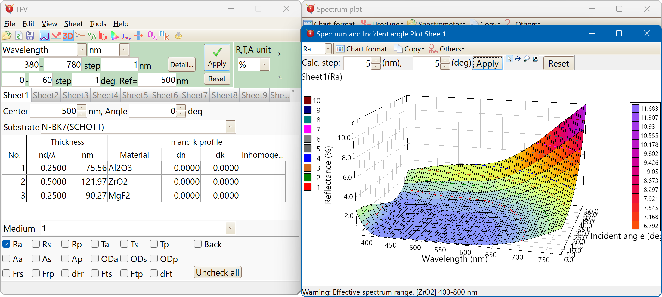
You can display a 3D graph with xy axes of spectrum and incident angle.
You can set the contour lines.
It is also possible to rotate and zoom with the mouse.
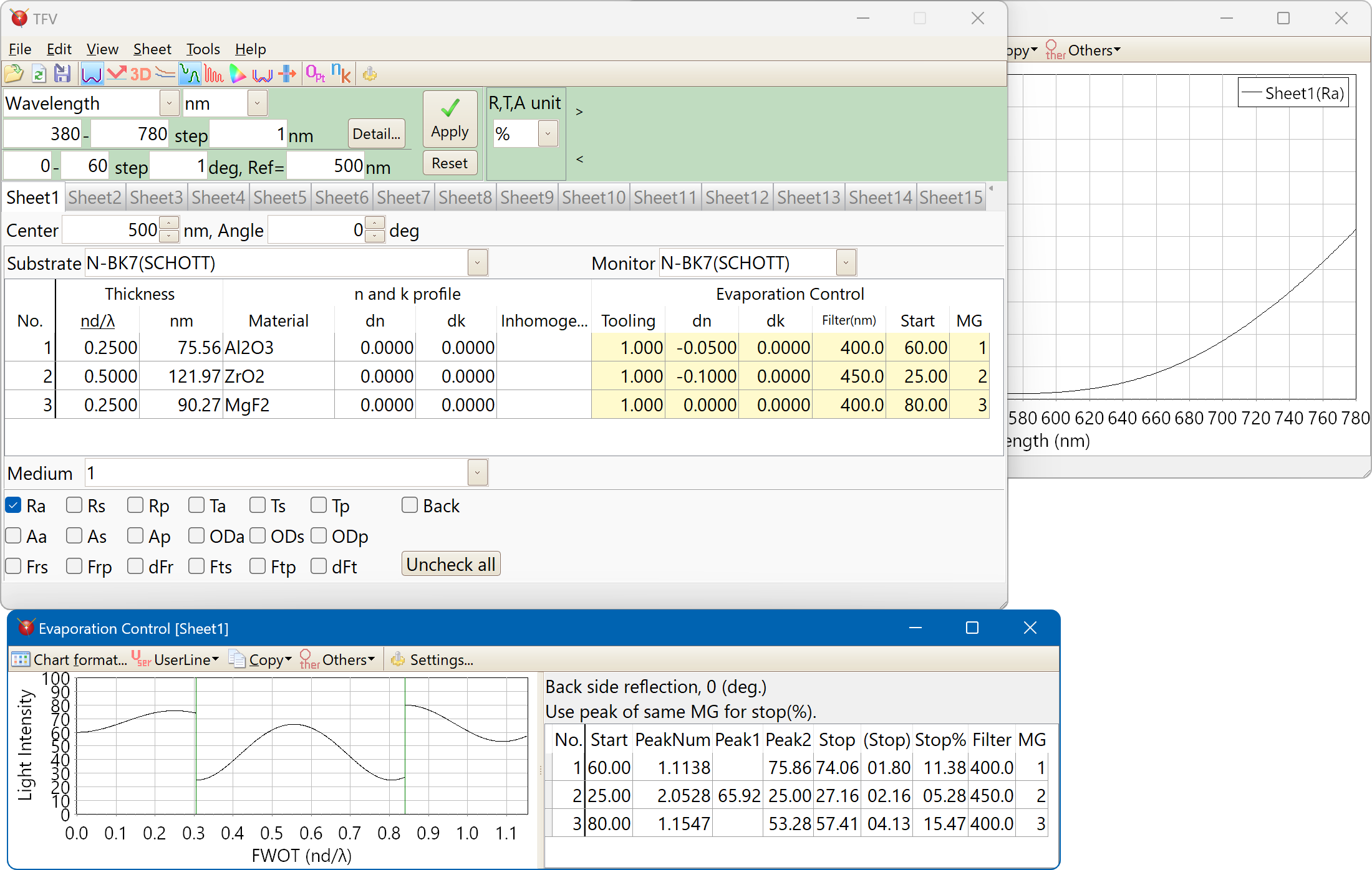
Optical monitor
Optical monitor simulation that considers the tooling factor and the in situ n and k is possible.
All layers information can be displayed simultaneously.
- Supporting type of monitoring system
-
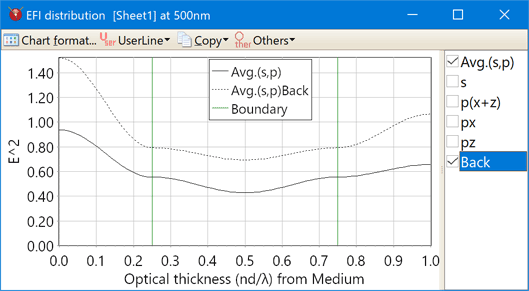
Electric field intensity
Each polarization of electric field can be displayed.
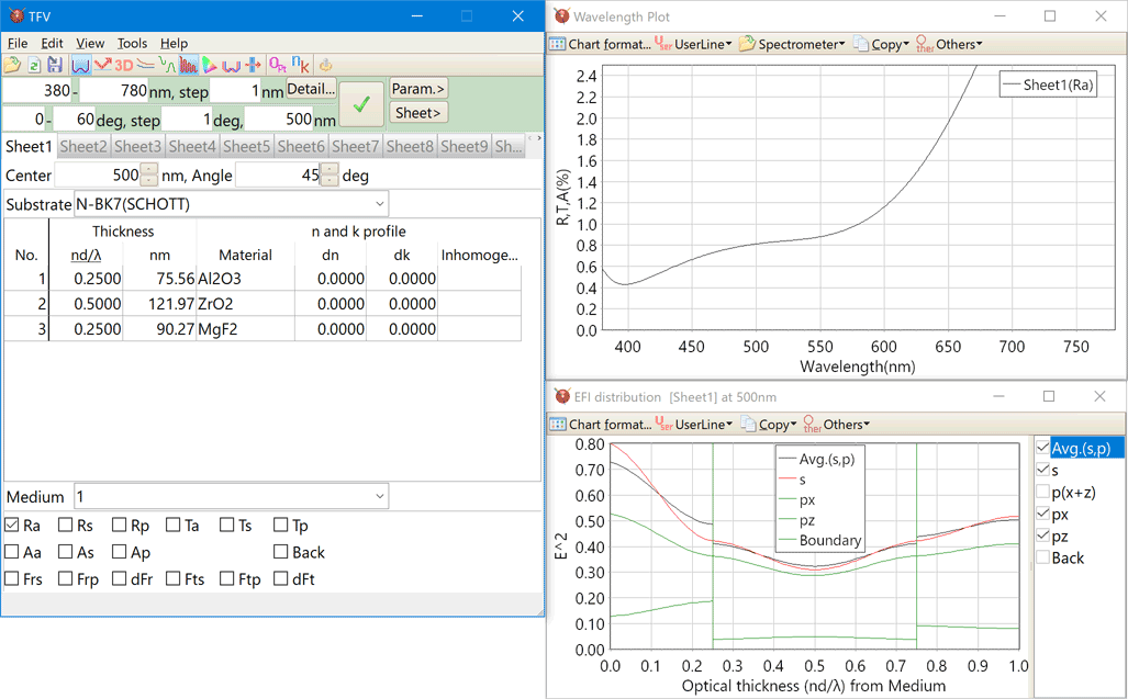
The front side and the reverse side electric fields can be displayed simultaneously.
Color calculation
Color difference can be calculated. For example between the two design or between front side and reverse side.
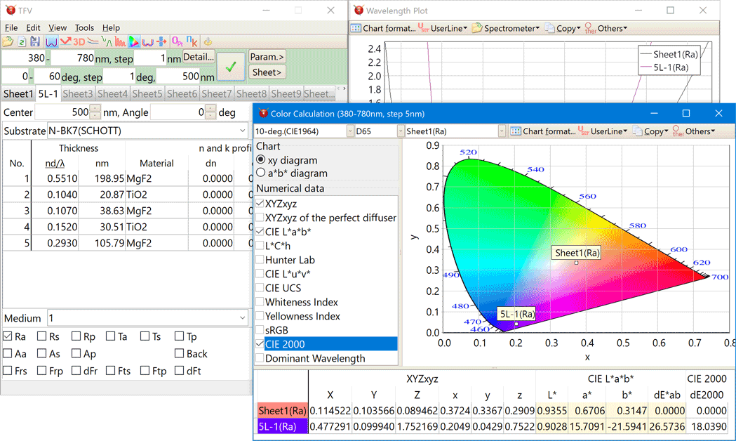
- Color system
-
XYZxy, CIE L*a*b*, L*C*h, Hunter Lab, L*u*v*, UCS, Whiteness Index, Yellowness Index, sRGB, CIE2000, Dominant Wavelength。
- Kind of the illuminant
-
A, B, C, D50, D55, D65, D75, E, F1, F2, F3, F4, F5, F6, F7, F8, F9, F10, F11, F12, ID50, ID65。
You can also register your own light source data as a csv file.
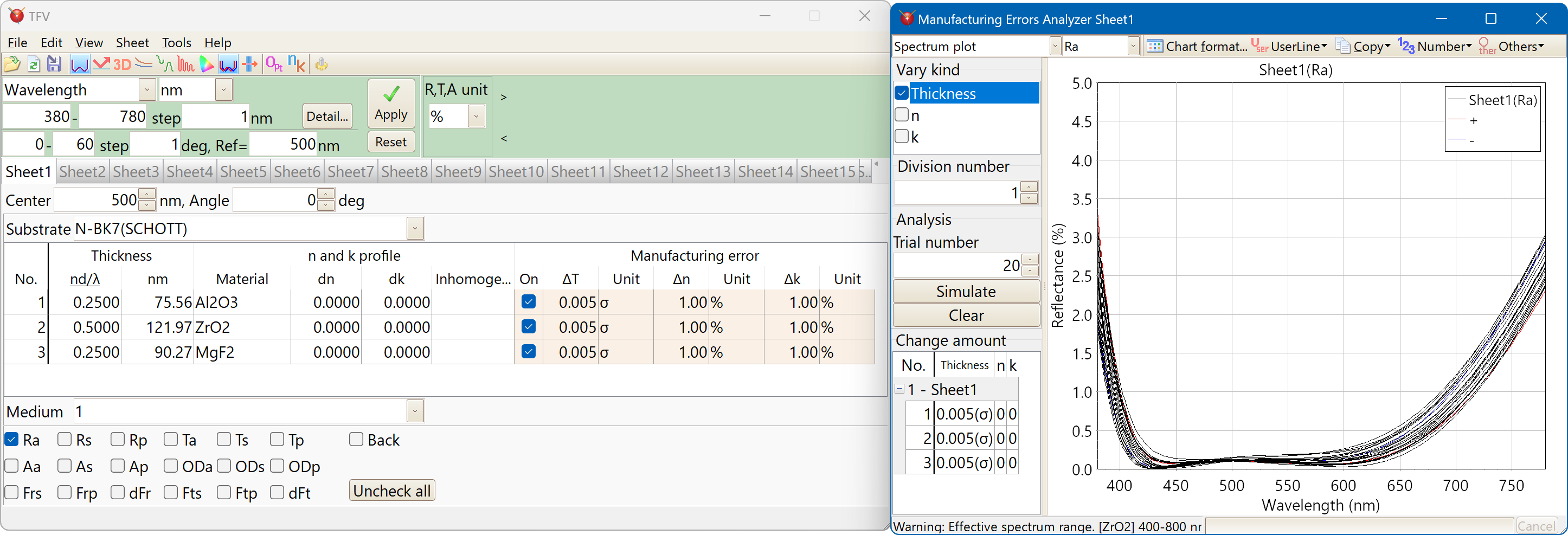
Manufacturing error
It is used to investigate how much the variation in film thickness, refractive index, and absorption coefficient affects the optical characteristics.
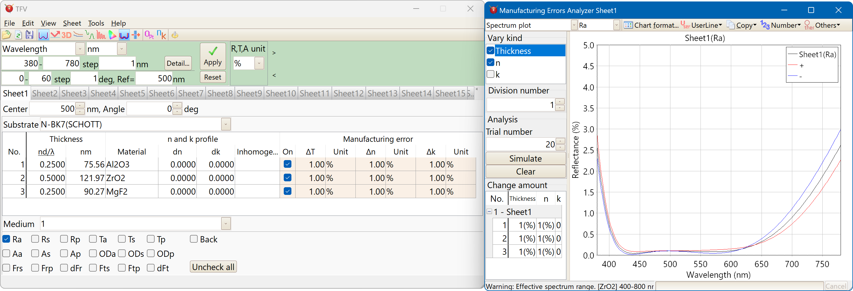
Monte Carlo simulation of spectral characteristics
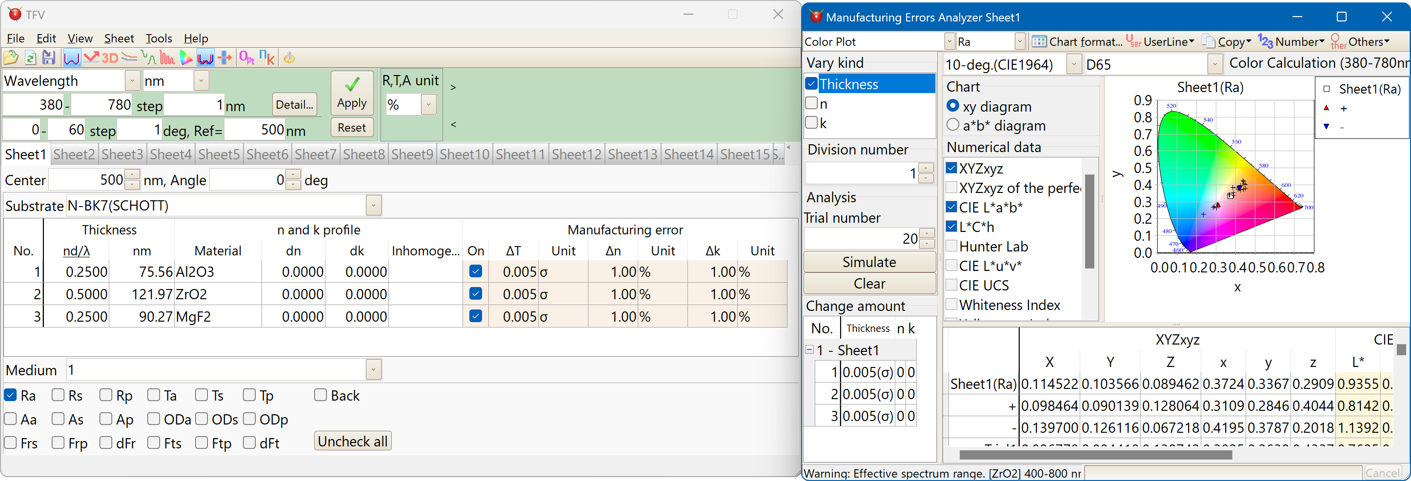
Monte Carlo simulation of color
You can specify the amount of change for each film thickness, refractive index, and absorption coefficient for each layer.
The amount of change can be selected from uniform distribution in absolute value, uniform distribution in%, and normal (Gaussian) distribution (σ).
We use the Mersenne Twister method to generate random numbers.
Group Delay
| Supported Types of Group Delay | |
|---|---|
| GD | Group Delay |
| GDD | Group Delay Dispersion |
| CDC | Chromatic Dispersion Coefficient |
| TOD | Third Order Dispersion |
| FOD | Fourth Order Dispersion |
| 5OD | Fifth Order Dispersion |
| Units |
|---|
| ps, fs |
In the calculation of group delay, differentiation also includes the optical constants (the dispersion formulas of n and k).
Numerical differentiation (finite difference) with large errors is not used.

Stack
It is possible to calculate the total when the film is attached to each side of multiple substrates (parallel plane substrates).
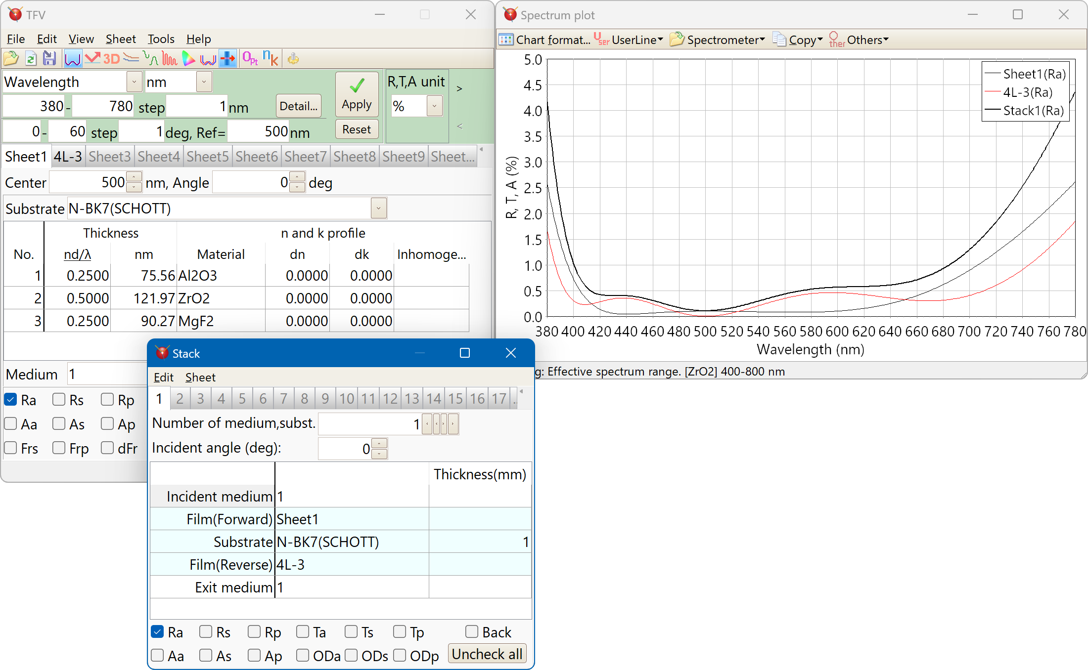
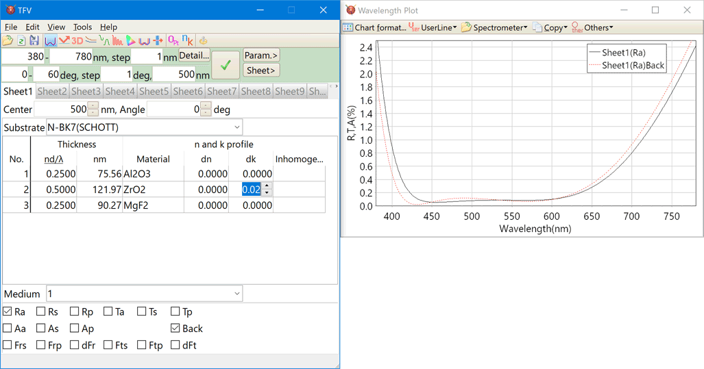
Reverse side
The results of front side and reverse side can be displayed simultaneously.
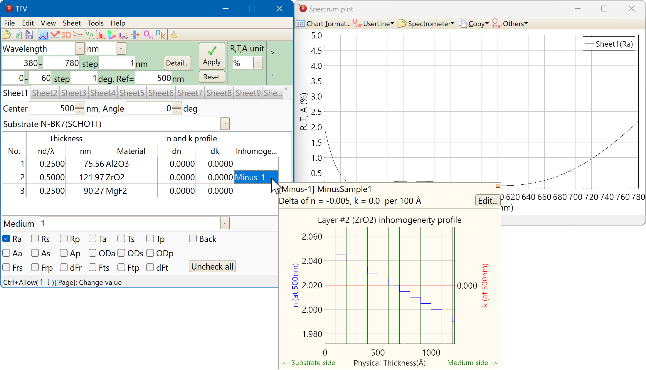
Inhomogeneity
If the mouse pointer is placed for a while on the "Inhomo..." cell, then the Inhomogeneity profile are displayed on the popup window.
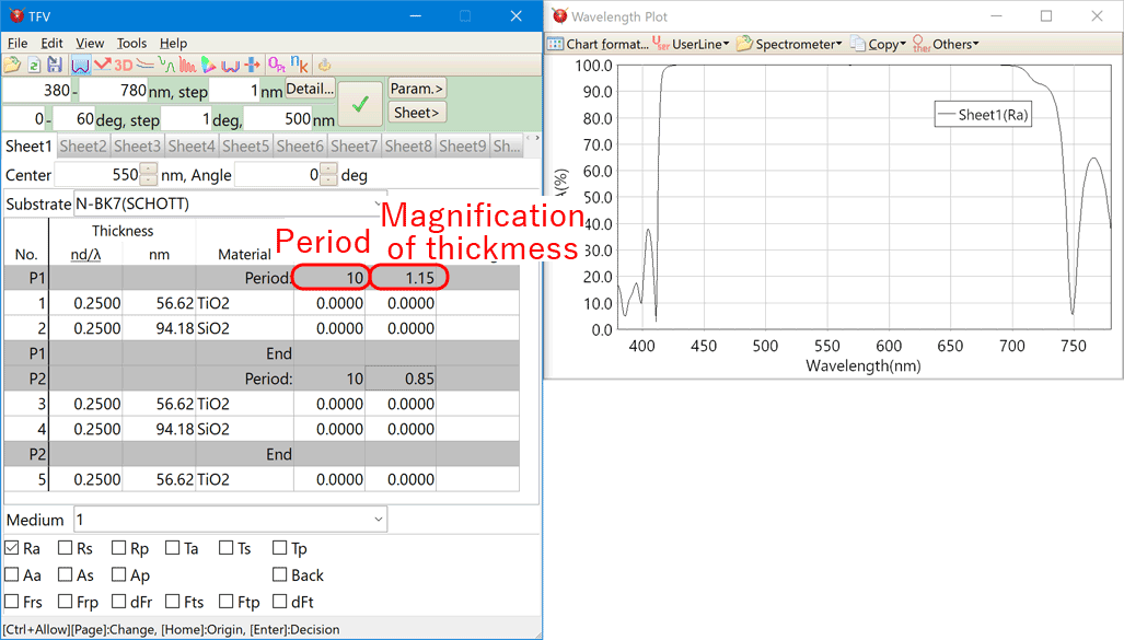
Periodic layer
Periodic layer can be displayed very clearly.
The magnification of the thickness each periodic layer can be set.
Optimization
Optimization(1) Standard mode
Standard mode has three search methods. Local search, global search and needle search.
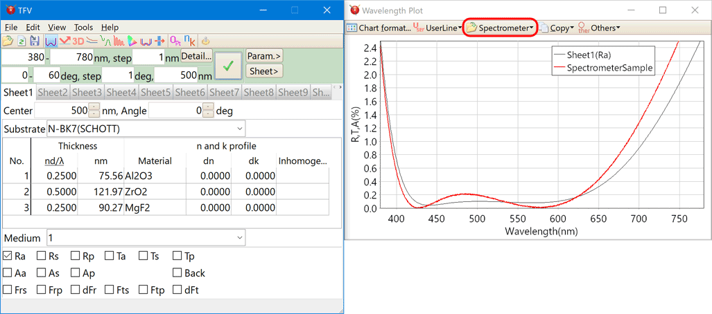
You can select the spectrometer data as the target, then simulate the difference between design and measured values easily.
- Local search
-
Local search is used Levenberg-Marquardt Method for optimization thickness.
- Global search
-
Global search is used Simulated Annealing Method and Levenberg-Marquardt Method.
- Needle search
- Needle search works by adding the needle-like layers into the design. After the needle-like layers have been added, the local search is used to optimization.
Optimization(2) Free-hand mode
When you trace with the mouse while holding down the left button near the selected series, then the shape of series is deformed. Optimize will be started automatically when you release the left button.n and k calculation for substrate and film
This function calculates n and k of a substrate or monolayer film from the measured values of spectral reflectance and spectral transmittance.
- Calculate refractive index of substrate without absorption
Calculate the refractive index of a substrate without films. It is used when there is no absorption on the substrate. A single-sided matte substrate or double-sided polished substrate is required. - Calculate refractive index, absorption coefficient and internal transmittance of substrate
Calculate the refractive index of a substrate without films. It is used when substrate has absorption. Both single-sided matte substrate and double-sided polished substrate are required. - n and k analysis of monolayer film
From the spectral reflectance and spectral transmittance, n, k and film thickness (d) of the film are analyzed by curve fitting to the dispersion formula.
Added an option to analyze only normal dispersion (dispersion in which the refractive index increases as the wavelength becomes shorter).
It is now possible to calculate each measurement data of "front reflection", "back reflection", and "transmission" even with different wavelengths and different measurement points. - Calculate n and k of monolayer metal film
Calculate n and k of the metal film from the front surface reflectance and the back-surface reflectance. The substrate must be thick enough and have a zero transmittance.
Spectrometer data
The spectrophotometer measured data files can be read on the chart.
If the measured data is relative value, you can convert the relative value into absolute value.
- Supported file format
-
Hitachi UV-Solutions files and UV1 files(*.UDSS, *.UDS, *.UDA, *.UV1),
Shimadzu SPC files,
Olympus-USPM files(*.dat, *.csv),
Jasco JWS files,
Ocean-Optics OOi-Base32 files,
csv files,
tab separated text files.
Dispersion
Substrate
- 1381 kinds of substrate are registered.
-
SCHOTT, OHARA, HOYA, SUMITA, HIKARI, CDGM
APEL, ZEONEX, PMMA, Polycarbonate, etc.
You can also register your own data.
Film material
- The following 33 types of materials are registered.
-
Ag, Al2O3, AL, Au, Cr, Cu, H2, H4, LaF3, M3, M3-RT, MgF2, Nb2O5, Nb2O5-RT, OH5, OH5-RT, OS50, OS50-RT, SiO2, Ta2O5, Ta2O5-RT, Ti, TiO2, Zn, ZnS, ZrO2, Cytop
-
Al2O3(KTM), HfO2(KTM), LaF3(KTM), Ti3O5(KTM), ZrO2(KTM), ZRT2(KTM)
KTM: Kyoto Thin-Film Materials Institute - You can also register your own data.
Kind of the dispersion formula
Dispersion formulas of refractive index n
-
Sellmeier
\[n(λ) = \sqrt{ 1 + {A_0λ^2 \over λ^2-A_3} + {A_1λ^2 \over λ^2-A_4} + {A_2λ^2 \over λ^2-A_5} } \] -
Sellmeier2
\[n(λ) = \sqrt{ 1 + A_0 + {A_1λ^2 \over λ^2-{A_3}^2} + {A_2 \over λ^2-{A_4}^2} } \]* A2 does not have λ2.
-
Sellmeier3
\[n(λ) = \sqrt{ 1 + {A_0λ^2 \over λ^2-A_4} + {A_1λ^2 \over λ^2-A_5} + {A_2λ^2 \over λ^2-A_6} + {A_3λ^2 \over λ^2-A_7} } \] -
Sellmeier4
\[n(λ) = \sqrt{ A_0 + {A_1λ^2 \over λ^2-A_3} + {A_2λ^2 \over λ^2-A_4} } \] -
Sellmeier5
\[n(λ) = \sqrt{ 1 + {A_0λ^2 \over λ^2-A_5} + {A_1λ^2 \over λ^2-A_6} + {A_2λ^2 \over λ^2-A_7} + {A_3λ^2 \over λ^2-A_8} + {A_4λ^2 \over λ^2-A_9} } \] -
SellmeierT1
\[n(λ) = \sqrt{ A_0 + {A_1λ^2 \over λ^2-A_2} } \] -
SellmeierT2
\[n(λ) = \sqrt{ A_0 + {A_1λ^2 \over λ^2-A_2} + A_3λ^2 } \] -
SellmeierX1
\[n(λ) = \sqrt{ 1 + {A_0λ^2 \over λ^2-{A_3}^2} + {A_1λ^2 \over λ^2-{A_4}^2} + {A_2λ^2 \over λ^2-{A_5}^2} } \] -
General1
\[n(λ) = \sqrt{ A_0 + A_1λ^2 + {A_2 \over λ^2} + {A_3 \over λ^4} + {A_4 \over λ^6} + {A_5 \over λ^8} + A_6λ^4 } \] -
General2 (Old Schott)
\[n(λ) = \sqrt{ A_0 + A_1λ^2 + {A_2 \over λ^2} + {A_3 \over λ^4} + {A_4 \over λ^6} + {A_5 \over λ^8} } \] -
Cauchy
\[n(λ) = A_0 + {A_1 \over λ^2} + {A_2 \over λ^4} \] -
Hartmann1
\[n(λ) = A_0 + {A_1 \over λ - A_2} \] -
Hartmann2
\[n(λ) = A_0 + {A_1 \over (λ - A_2)^2} \] -
Herzberger
\[n(λ) = A_0 + A_1 λ^2 + {A_2 \over (λ^2 - 0.168^2)} + {A_3 \over (λ^2 - 0.168^2)^2} \] -
Herzberger2
\[n(λ) = A_0 + {A_1 \over (λ^2 - 0.028)} + {A_2 \over (λ^2 - 0.028)^2} + A_3 λ^2 + A_4 λ^4 + A_5 λ^6 \] -
QUAD
\[n(λ) = A_0 + {A_1 \over λ^2} \] -
QUADSK
\[n(λ) = A_0 + A_1 λ + A_2 λ^2 \] -
Conrady
\[n(λ) = A_0 + {A_1 \over λ} + {A_2 \over λ^{3.5}} \] -
Handbook1 (Handbook of Optics)
\[n(λ) = \sqrt{ A_0 + {A_1 \over (λ^2 - A_2)} - A_3λ^2 } \] -
Handbook2 (Handbook of Optics)
\[n(λ) = \sqrt{ A_0 + { A_1 λ^2 \over (λ^2 - A_2)} - A_3λ^2 } \] -
Extended (ZEMAX)
\[n(λ) = \sqrt{ A_0 + A_1λ^2 + {A_2 \over λ^2} + {A_3 \over λ^4} + {A_4 \over λ^6} + {A_5 \over λ^8} + {A_6 \over λ^{10}} + {A_7 \over λ^{12}} } \] -
Extended2 (ZEMAX)
\[n(λ) = \sqrt{ A_0 + A_1λ^2 + {A_2 \over λ^2} + {A_3 \over λ^4} + {A_4 \over λ^6} + {A_5 \over λ^8} + A_6 λ^4 + A_7 λ^6 } \] -
Extended3 (ZEMAX)
\[n(λ) = \sqrt{ A_0 + A_1λ^2 + A_2λ^4 + {A_3 \over λ^2} + {A_4 \over λ^4} + {A_5 \over λ^6} + {A_6 \over λ^8} + {A_7 \over λ^{10}} + {A_8 \over λ^{12}} } \] -
Buchdahl
\[n(λ) = A_0 + A_1 ω(λ) + A_2 ω(λ)^2 \] \[ω(λ) = { λ - A_3 \over 1 + 2.5(λ - A_3) } \] -
DRUDE
\[{n^2}(λ) - {k^2}(λ) = A_0 - { A_1 {A_2}^2 λ^2 \over λ^2 + {A_2}^2 } \] -
LorentzianK
\[n(λ) = \sqrt{ A_0 + {k^2}(λ) + A_1 λ^2 {(λ^2 - {A_2}^2) \over (λ^2 - {A_2}^2)^2 + {A_3}^2 λ^2 } } \] -
Forouhi-Bloomer
\[n(E) = n(∞) + {B_0E+C_0 \over E^2 - BE + C} \] \[B_0 = {A \over Q}{({-B^2 \over 2} + E_gB - {E_g}^2 + C)} \] \[C_0 = {A \over Q}{\left(({E_g}^2 + C){B \over 2}-2E_gC\right)} \] \[Q = {1 \over 2}{(4C-B^2)}^{1 \over 2} \] \[E= {{hc} \over λ} \]h: Planck's constant, c: Light speed, The unit of E: eV.
n(∞), Eg, A, B, C: Material constants(parameters of the dispersion formula) -
A0, A1, A2, A3, A4, A5, A6, A7, A8, A9: material constants.
The unit of λ is μm (excluding Forouhi-Bloomer).
Dispersion formulas of absorption coefficient k
-
Sellmeier
\[k(λ) = {\biggl[ n(λ) \biggl(B_0 λ + {B_1 \over λ} + {B_2 \over λ^3} \biggr) \biggr]}^{-1} \] -
Cauchy
\[k(λ) = B_0 + {B_1 \over λ^2} + {B_2 \over λ^4} \] -
Exponential
\[k(λ) = B_0 \cdot exp(B_1 λ^{-1}) \] -
QUADSK
\[k(λ) = B_0 + B_1 λ + B_2 λ^2 \] -
DRUDE
\[2n(λ)k(λ) = { A_1 A_2 λ^3 \over λ^2 + {A_2}^2 } \] -
LorentzianK
\[k(λ) = \sqrt{ {0.5 \over n(λ)} \cdot {A_1 A_3 λ^3 \over (λ^2 - {A_2}^2)^2 + {A_3}^2 λ^2 } } \] -
Forouhi-Bloomer
\[k(E) = {A(E-E_g)^2 \over {E^2 - BE + C}} \] \[E= {{hc} \over λ} \]h: Planck's constant, c: Light speed, The unit of E: eV.
Eg, A, B, C: Material constants(parameters of the dispersion formula) -
B0, B1, B2: material constants.
The unit of λ is μm (excluding Forouhi-Bloomer).
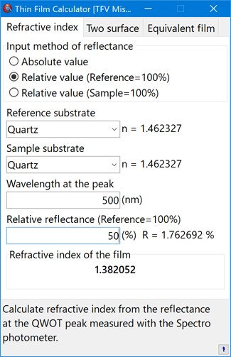
Misc calculator
The misc calculator is the simple calculation tool of thin film.
Refractive index
Calculate refractive index from the reflectance at the QWOT peak measured with the spectrophotometer.
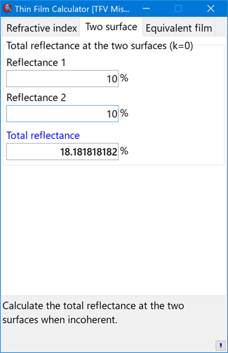
Two surface
Calculate the total reflectance at the two surfaces when incoherent.
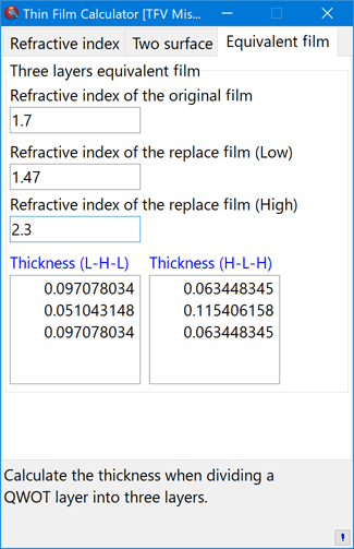
Equivalent film
Calculate the thickness when dividing a QWOT layer into three layers.